How do you calculate confidence intervals for a prediction?

This is a question that comes up frequently in forecasting. But it is surprisingly hard to answer, because it boils down to predicting how accurate a forecast will be – a prediction about a prediction. Prediction squared.

One approach is to base the estimate on past errors in similar situations. This method is used for example by the National  Institute of Statistics and Economic Studies (INSEE) in France, who wrote  that “the distribution of forecasting errors calculated from past exercises is a reliable indicator of the distribution of future errors and hence of the uncertainty  surrounding a given forecast” (see this research paper).

But this assumes that the new data will follow a familiar pattern – which may not be the case if for example you are trying to predict the effect of a novel economic policy, or a new drug, or climate change.

Another approach is to randomly perturb model parameters. But this has problems of its own.

To illustrate this, consider a simple linear model x(t) = k*t + x0, and suppose we want to predict the state at time t=1 based on an observation at t=0. Without loss of generality we can set the expected slope of the model to k=0, so the prediction is a persistence forecast: x1 = x0 (here x1 = x(1) and x0 = x(0)). Treating errors as random variables, then (in terms of variance) the error in the prediction, relative to the observation, will be the sum of the variance of the initial and final observational errors (see note below for details).

Schematic for error in persistence model prediction. Black points are initial and final observations, with error bounds. Red line is true state. Blue dashed line is model prediction. Note assumption that persistence model is correct.
Schematic for error in persistence model prediction. Black points are initial and final observations, with error bounds. Red line is true state (assumed to remain constant). Blue dashed line is prediction based on persistence model. Because the model is correct, all error is due to observations.

This makes sense since we are assuming the model is perfect, so all error comes from the observations. But in the real world, model error is not usually zero! Observational error is only part of the puzzle. So how do we estimate the contribution of model error?

As mentioned above, a typical approach is to perturb the parameters of the model by some reasonable amount, or do a Monte Carlo over a range of parameter values. (See paper on ensemble forecasting with model error.) For our simple linear model, a Monte Carlo simulation using a normal distribution around 0 with variance w for the parameter k would then give an ensemble of model predictions, with the same variance of w. Again this error will add to the error due to the observations.

This all sounds very logical and scientific, and versions of this approach are used by everyone from central bankers to weather forecasters. But again there is a catch, because the answer will depend on the parameter range that we selected. In other words, we can get whatever answer we want by choosing the range.

Of course, one can argue for a particular range – but if we are forecasting a new situation, we can’t base the estimate reliably on past data.

And there is an even more intractable issue – which is that the prediction error may be due not to parameter error, but to model structure. What if the actual system is not linear? (It probably isn’t.)

The ultimate problem is that the frequentist approach to statistics breaks down completely in forecasting – it relies on analyzing data, but the whole point of forecasting is that there is no data to measure (otherwise you could just measure it and not bother with the forecast).

Fortunately there is a solution, or at least an intellectually consistent method, which is to take a Bayesian approach. Unlike the commonly-taught frequentist approach, which treats probabilities as a measure of the frequency of observed events, the Bayesian approach interprets probabilities as a measure of degrees of belief. And in forecasting, confidence intervals ultimately are a measure of one’s confidence in the model.

In the case of our simple model, the idea is to come up with an initial confidence interval, based for example on previous experience, but see it as an estimate only, and refine it as more data comes in.

Of course this requires admitting that the confidence interval relies on subjective estimates. However doing so can help to avoid another problem in mathematical modelling, which is the tendency of frequentist error estimates to ignore the effect of context and prior information. Read our article on the BayesianOpinionator.

Notes:

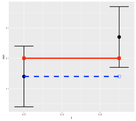
For the simple linear model case, prediction error is the sum of the initial and final errors. We’ll use x to denote predictions, y for the true state, z for observations, and e for observational errors.

Suppose that the observed initial condition z0 is observed with an error e0, and the observed final point z1 has an error e1. So the true initial condition is y0 = z0 + e0, and the true final state is y1 = z1+ e1.

If we assume there is no model error, then y1 = y0. It follows that the difference between the forecast x1 = z0 and the observed final state z1 is:

error = z1- z0 = y1 – e1 – y0 + e0 = e0 – e1.

If the errors are assumed to be normal with variance v0 and v1, then the forecast error has variance v0 + v1 (variance is additive), which allows us to determine confidence intervals. So for example a 95% confidence interval would be +/-1.96 times the standard deviation.

If we assume that model error contributes an error at time 1 with variance w1, then again the variances are additive, and the total will increase to v0 + v1 + w1.

The BayesianOpionionator

I recently finished Robert Matthew’s excellent book Chancing it: The laws of chance – and what they mean for you. One of the themes of the book is that reliance on conventional statistical methods, such as the p-value for measuring statistical significance, can lead to misleading results.

An example provided by Matthews is a UK study (known as The Grampian Region Early Anistreplase Trial, aka GREAT) from the early 1990s of clot-fighting drugs for heart attack patients, which appeared to show that administering the drugs before they reached hospital reduced the risk of death by as much as 77 percent. The range of the effect was large, but was still deemed statistically significant according to the usual definition. However subsequent studies showed that the effect of the drug was much smaller.

Pocock and Spiegelhalter (1992) had already argued that prior studies suggested a smaller effect. They used a Bayesian approach in which a prior belief is combined with the new data to arrive at a posterior result. The impact of a particular study depends not just on its apparent size, but also on factors such as the spread. Their calculations showed that the posterior distribution for the GREAT study was much closer to the (less exciting) prior than to the experimental results. The reason was that the experimental spread was large, which reduced its impact in the calculation.

Given the much-remarked low degree of reproducibility of clinical studies (in the US alone it has been estimated that approximately US$28,000,000,000 is spent on preclinical research that is not reproducible) it seems that a Bayesian approach could prove useful in many cases. To that end, we introduce the BayesianOpinionator, a web app for incorporating the effect of prior beliefs when determining the impact of a statistical study.

Screenshot of the Bayesian Opionator
Screenshot of the BayesianOpinionator

The data for the BayesianOpinionator app is assumed to be in the form of a comparison between two cases, denoted null and treated. For example in a clinical trial the treated case could correspond to a patient population who are treated with a particular drug, and the null case would be a comparison group that are untreated. As mentioned already, a common problem with such studies is that they produce results which appear to be statistically significant, but later turn out to be caused by a fluke. In this case the BayesianOpinionator will help to determine how seriously the results should be taken, by taking prior beiefs and data into account. The method works by representing data in terms of binomial distributions, which as seen below lead to a simple and intuitive way of applying weights to different effects in order to gauge their impact.

The New Data page is used to input the trial results, which can be in a number of different forms. The first is a binary table, with the two options denoted Pos and Neg – for example these could represent fatalities versus non-fatalities. The next is a probability distribution, where the user specifies the mean and the standard deviation of the probability p of the event taking place for each case. Finally, studies are sometimes reported as a range of the odds ratio (OR). The odds for a probability p is defined as p/1-p, so is the ratio of the chance of an event happening to the chance of it not happening. The OR is the odds of the treated case, divided by the odds of the null case. An OR of 1 represents no change, and an OR range of 0.6 to 1 would imply up to 40 percent improvement. Once the odds range is specified, the program searches for a virtual trial which gives the correct range. (The user is also asked to specify a null mean, otherwise the result is underdetermined.)

In all cases, the result is a binomial distribution for the treated and null cases, with a probability p that matches the average chance of a positive event taking place. Note that the problems studied need not be limited to binary events. For example, the data could correspond to diameter growth of a tumor with or without treatment, from a scale of 0 to 1. Alternatively, when data is input using the probability range option, a range can be chosen to scale p between any two end points, which could represent the minimum and maximum of a particular variable. In other words, while the binomial distribution is based on a sequence of binary outcomes, it generalises to continuous cases while retaining its convenient features.

In the next page Prior, the user inputs the same type of information to represent their prior beliefs about a trial. Again, this information is used to generate binomial distributions for the prior case. Finally, the two sets are pooled together in order to give the posterior result on the next page. The posterior is therefore literally the sum of the prior and the new data.

The next page, Odds, shows how the new results compare with the prior in terms of impact on the posterior. The main plot shows the log-OR distribution, which is approximately normal. A feature of the odds ratio is that it allows for a simplified representation within the Bayesian framework. The posterior distribution can be calculated as the weighted sum of the prior and the new data. The weights are given in table form, and are represented graphically by the bubble plot in the sidebar. The size of the bubbles represents spread of log-OR, while vertical position represents weight of the data, with heavy at the bottom.

As shown by Matthews (see this paper), the log-OR plot allows one to determine a critical prior interval (CPI) which can be viewed as the minimum necessary in order for the new result to be deemed statistically significant (i.e. has a 95 percent chance of excluding the possibility of no effect). If the CPI is more extreme than the result, this implies that the posterior result will not be significant unless one already considers the CPI to be realistic. For clinical trials, which for ethical reasons assume no clear advantage between the null and treated cases, the CPI acts as a reality check on new results, because if the results are very striking it shows how flexible the prior needs to be in order to see them as meaningful.

The BayesianOpinionator Shiny app can be accessed here.

Model Misuse: Applying hypothesis testing to simulated data from in-silico cardiac models

In the previous blog there was an interesting link to a report by Yaron Hollander on the use and abuse of models in transport forecasting.  His description of abuse of models can be seen in many sectors including the life sciences where it is arguably a bigger issue. Why? Other sectors have to some degree acknowledged the concept of structural uncertainty, which is a taboo subject for, most not all, modelers within the life sciences sector.  By acknowledging there is a problem modelers within the other sectors have at least moved beyond the denial phase, the first phase of an addiction problem.  This does not seem to be the case for most life sciences modelers.  A typical example of this can be seen in a recent article by Zhou et al. from the University of Oxford which explores the mechanisms, through use of modelling and simulation, behind certain biological phenomena in cardiac myocytes termed alternans (alternating long and short action potentials)…

In the article, Zhou et al., claim that the mathematical/computational model being used within the study is the “gold standard” and has been “extensively validated”.  Declaring a model as being the gold standard and extensively validated gives a licence to models being used to answer many questions which the model has not been tested for which will lead to all sorts of misuse of a model. Indeed the type of model used by Zhou et al. can never truly be tested due to its scale: 10’s of variables and 100’s of parameters.  Such large models, which also include extensive non-linear functions, are almost impossible to test because they are so flexible. Thus, using such models for the type of analysis Zhou et al. conducted can be considered a classic example of model misuse. The authors applied the following analysis (more detail can be found in the article):

  • A population of models is created by generating 10000 parameter sets by perturbing a subset of model parameters
  • Of these a subset (~2500) are deemed acceptable according to some criteria
  • Each of these parameter sets are then used to explore the alternan phenomena
  • Parameter sets are then grouped by how they answer the following questions:
    1. Does a parameter set produce alternans or not
    2. Are the alternans eye or folk type
  • Finally statistical tests are performed to ascertain whether the distributions of parameters are different between the groups created.

In essence they are applying statistical tests to simulated data, which has been discussed within ecology as something that should not be done.  White et al. provide two reasons why statistical significance tests should not be used to interpret simulation results of which the first is most relevant here as the second is more a philosophical debate to some degree.  The first reason revolves around power calculations: probability that a test correctly rejects the null hypothesis when the alternative is true. One of the key components of a power calculation is sample size! In brief, by using such a large sample size, numbers of simulations, Zhou et al. have powered their study to be able to detect the smallest of differences between groups.  Indeed Zhou et al. can control the sample size and thus control the results of a statistical test; they could be accused of p-hacking. This brings into question the results seen by Zhou et al. In addition to the misuse of statistical hypothesis testing there is another more worrying issue about the first step of the approach: using large flexible models to explain variability in a dependent variable, measured experimentally, by varying a subset of model parameters.  An obvious question is which parameters should be varied in such large models given how flexible they are? Furthermore, the bigger issue around structural uncertainty still hasn’t been addressed with such an approach.  What consequences could these issues have? It will lead to a high number of false positives and waste experimental resources chasing hypotheses that were not worthwhile.

Finally on an even more cautionary note, if the type of approach, described by Zhou et al., were used to develop biomarkers and to guide clinical trials then this is likely to increase clinical trial failure rates rather than improve them. In an era where people within the healthcare industry are looking at systems approaches, real care must be taken as to what approaches are actually used within the industry. As modelers our duty is to remain questioning and skeptical.

Model abuse isn’t unique to transport forecasting …

By David Orrell

Yaron Hollander from the consultancy firm CT Think! published an interesting report on the use and abuse of models in transport forecasting. The report, which was summarised in Local Transport Today magazine, cited ten different problems, which apply not just to transport forecasting but to other areas of modelling as well:

1. Referring to model outputs when discussing impacts that weren’t modelled

2. Presenting modellers’ assumptions as if they were forecasts

3. “Blurring the caveats” provided by modellers when copying model outputs from a technical report to a summary report

4. Using model outputs at a level of geographical detail that does not match the capabilities of the model or the data that were used to develop it

5. Reporting estimated outcomes and benefits with a high level of precision, without sufficient commentary on the level of accuracy

6. Presenting a large number of model runs or scenarios with limited interpretation of each run, as if this gives a good understanding of the impacts of the investment

7.Avoiding clear statements about how unsure we really are about the future pace of social and economic trends

8. Testing the sensitivity of the results to some inputs as if it helps us understand the sensitivity to all inputs

9. Discussing uncertainty in forecasts as if all it could do is change the scale of the impacts, ignoring possible impacts of a very different nature

10. Avoiding discussions about the history of the model itself, which sometimes goes many years back and includes features that the current owners do not understand

I was invited along with several other people to give a response, which is included below. Although I didn’t mention computational biology as one of the areas affected, it certainly isn’t immune!

Here is the full response, which was published in LTT (paywall):

Forget complexity, models should be simple

The report by Yaron Hollander accurately identifies a number of different types of “model abuse” in transport forecasting. I would just add a couple of comments. One is that these problems are not unique to transport, but are common in many other areas of forecasting as well, as I found while researching my 2007 book The Future of Everything: The Science of Prediction. This is especially the case when the incentives of the forecasters are entwined with the outcome of the predictions.

An example from the early 1980s was a paper by Will Keepin and Brian Wynne which showed that a model used by nuclear scientists to predict future energy requirements vastly overestimated the need for nuclear power plants, as well as the number of nuclear scientists needed to design them. In finance, many of the models used to value complex derivatives are less about accuracy, than about justifying risky trades. This is why two leading quants, Paul Wilmott and Emanuel Derman, wrote their own Modelers’ Hippocratic Oath. Even apparently objective areas such as weather forecasting are not immune from model abuse. I would argue that techniques such as ensemble forecasting, which involves running many forecasts from perturbed initial conditions, are an example of Hollander’s point 8: “Testing the sensitivity of the results to some inputs as if it helps us understand the sensitivity to all inputs.”

The author notes that public consultation is a promising solution, however one of the attractive features of mathematical models, if defending them is the aim, is exactly the fact that they can only be understood by a relatively small number of experts (who often come from the same area). Mathematical equations can seem imposing to those outside the field, which grants a degree of immunity from external scrutiny. So the public needs access to experts who are willing to point out the flaws in models.

Mathematical modellers are always happy to build complex models of any system and attempt to make predictions. But we need more studies which attempt to answer a different forecasting question: based on past experience, and knowledge of a model’s strengths and weaknesses, are predictions based on the model likely to be accurate? The answer in many cases is “probably not” – which has implications for decision-makers. This does not of course mean that we should do away with modelling, only that we should concentrate on simple models, where the assumptions and parameters are well-understood, and be realistic about the uncertainty involved.

Complexity versus simplicity in relating tumour size change to survival in oncology drug development

Every pharmaceutical company would like to be able to predict the survival benefit of a new cancer treatment compared to an existing treatment as early as possible in drug development.  This quest for the “holy grail” has led to tremendous efforts from the statistical modelling community to develop models that link variables related to change in disease state to survival times.  The main variable of interest, for obvious reasons, is tumour size measured via imaging.  The marker derived from imaging is called the Sum of Longest Diameters (SLD).  It represents the sum of longest diameters of target lesions, which end up being large lesions that are easy to measure.  Therefore the marker is not representative of the entire tumour burden within the patient.  However, a change within the first X weeks of treatment in SLD is used within drug development to make decisions regarding whether to continue the development of a drug or not.  Therefore, changes in SLD have been the interest of most, if not all, statistical models of survival.

There are two articles that currently analyse the relationship between changes in SLD and survival in quite different ways across multiple studies in non-small cell lung cancer.

The first approach (http://www.ncbi.nlm.nih.gov/pubmed/19440187) by the Pharmacometrics (pharmaco-statistical modelling) group within the FDA involved quite a complex approach.  They used a combination of semi-parametric and parametric survival modelling techniques together with a mixed modelling approach to develop their final survival model.  The final model was able to fit to all past data but the authors had to generate different parameter sets for different sub-groups.  The amount of technical ability required to generate these results is clearly out of the realms of most scientists and requires specialist knowledge.  This approach can quite easily be defined as being complex.

The second approach (http://www.ncbi.nlm.nih.gov/pubmed/25667291) by the Biostatistics group within the FDA involved a simple plotting approach!  In the article the authors categorise on-treatment changes in SLD using a popular clinical approach to create drug response groups.  They then assess whether the ratio of drug response between the arms of clinical studies related to the final outcome of the study.  The outcomes of interest were time to disease progression and survival.  The approach actually worked quite well!  A strong relationship was found between ratio of drug response and the differences in disease progression.  Although not as strong, the relationship to survival was also quite promising.  This approach simply involved plotting data and can be clearly done by most if not all scientists once the definitions of variables are understood.

The two approaches are clearly very different when it comes to complexity: one involved plotting while the other required degree-level statistical knowledge!  It could also be argued that the results of the plotting approach are far more useful for drug development than the statistical modelling approach as it clearly answers the question of interest.  These studies show how sometimes thinking about how to answer the question through visualisation and also taking simple approaches can be incredibly powerful.

When is a model a black box?

One of the issues which comes up frequently with mathematical modelling is the question of whether a model is a “black box”. A model based on machine learning, for example, is not something you can analyse just by peering under the hood. It is a black box even to its designers.

For this reason, many people feel more comfortable with mechanistic models which are based on causal descriptions of underlying processes. But these come with their problems too.

For example, a model of a growing tumour might incorporate a description of individual cells, their growth dynamics, their interactions with each other and the environment, their access to nutrients such as oxygen, response to drugs, and so on. A 3D model of a heart has to incorporate additional effects such as fluid dynamics, electrophysiology, and so on. In principal, all of these processes can be written out as mathematical equations, combined into a huge mathematical model, and solved. But that doesn’t make these models transparent.

One problem is that each component of the model – say an equation for the response of a cell to a particular stimulus – is usually based on approximations and is almost impossible to accurately test. In fact there is no reason to think that complex natural phenomena can be fit by simple equations at all – what works for something like gravity does not necessarily work in biology. So the fact that something has been written out as a plausible mechanistic process does not tell us much about its accuracy.

Another problem is that any such model will have a huge number of adjustable parameters. This makes the model very flexible: you can adjust the parameters to get the answer you want. Models are therefore very good at fitting past data, but they often do less well at predicting the future.

A complex mechanistic model is therefore a black box of another sort. Although we can look under its hood, and see all the working parts, that isn’t very useful, because these models are so huge – often with hundreds of equations and parameters – that it is impossible to spot errors or really understand how they work.

Of course, there is another kind of black box model, which is a model that is deliberately kept inside a black box – think for example of the trading algorithms used by hedge funds. Here the model may be quite simple, but it is kept secret for commercial reasons. The fact that it is a closely-guarded secret probably just means that it works.