The Minsky model was developed by Steve Keen as a simple macroeconomic model that illustrates some of the insights of Hyman Minsky. The model takes as its starting point Goodwin’s growth cycle model (Goodwin, 1967), which can be expressed as differential equations in the employment rate and the wage share of output.
The equations for Goodwin’s model are determined by assuming simple linear relationships between the variables (see Keen’s paper for details). Changes in real wages are linked to the employment rate via the Phillips curve. Output is assumed to be a linear function of capital stock, investment is equal to profit, and the rate of change of capital stock equals investment minus depreciation.
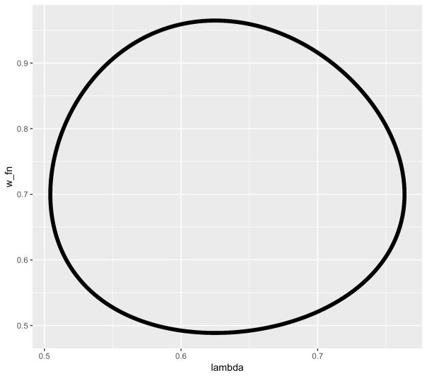
The equations in employment rate and wage share of output turn out to be none other than the Lotka–Volterra equations which are used in biology to model predator-prey interaction. As employment rises from a low level (like a rabbit population), wages begin to climb (foxes), until wages becomes too high, at which point employment declines, followed by wages, and so on in a repeating limit cycle.
In order to incorporate Minsky’s insights concerning the role of debt finance, a first step is to note that when profit’s share of output is high, firms will borrow to invest. Therefore the assumption that investment equals profit is replaced by a nonlinear function for investment. Similarly the linear Phillips curve is replaced by a more realistic nonlinear relation (in both cases, a generalised exponential curve is used). The equation for profit is modified to include interest payments on the debt. Finally the rate of change of debt is set equal to investment minus profit.
Together, these changes mean that the simple limit cycle behavior of the Goodwin model becomes much more complex, and capable of modelling the kind of nonlinear, debt-fueled behavior that (as Minsky showed) characterises the real economy. A separate equation also accounts for the adjustment of the price level, which converges to a markup over the monetary cost of production.
So how realistic is this model? The idea that employment level and wages are in a simple (linear or nonlinear) kind of predator-prey relation seems problematic, especially given that in recent decades real wages in many countries have hardly budged, regardless of employment level. Similarly the notion of a constant linear “accelerator” relating output to capital stock seems a little simplistic. Of course, as in systems biology, any systems dynamics model of the economy has to make such compromises, because otherwise the model becomes impossible to parameterise. As always, the model is best seen as a patch which captures some aspects of the underlying dynamics.
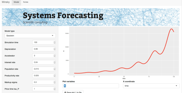
In order to experiment with the model, I coded it up as a Shiny app. The model has rate equations for the following variables: capital K, population N, productivity a, wage rate w, debt D, and price level P. (The model can also be run using Keen’s Minsky software.) Keen also has a version that includes an explicit monetary sector (see reference), which adds a few more equations and more complexity. At that point though I might be tempted to look at simpler models of particular subsets of the economy.
References
Goodwin, Richard, 1967. A growth cycle. In: Feinstein, C.H. (Ed.), Socialism, Capitalism and Economic Growth. Cambridge University Press, Cambridge, 54–58.
Keen, S. (2013). A monetary Minsky model of the Great Moderation and the Great Recession. Journal of Economic Behavior and Organization, 86, 221-235.