Monthly Archives: September 2016

The exponential growth effect

A common critique of biologists, and scientists in general, concerns their occasionally overenthusiastic tendency to find patterns in nature – especially when the pattern is a straight line. It is certainly notable how, confronted with a cloud of noisy data, scientists often manage to draw a straight line through it and announce that the result is “statistically significant”.

Straight lines have many pleasing properties, both in architecture and in science. If a time series follows a straight line, for example, it is pretty easy to forecast how it should evolve in the near future – just assume that the line continues (note: doesn’t always work).

However this fondness for straightness doesn’t always hold; indeed there are cases where scientists prefer to opt for a more complicated solution. An example is the modelling of tumour growth in cancer biology.

Tumour growth is caused by the proliferation of dividing cells. For example if cells have a cell cycle length td, then the total number of cells will double every td hours, which according to theory should result in exponential growth. In the 1950s (see Collins et al., 1956) it was therefore decided that the growth rate could be measured using the cell doubling time.

In practice, however, it is found that tumours grow more slowly as time goes on, so this exponential curve needed to be modified. One variant is the Gompertz curve, which was originally derived as a model for human lifespans by the British actuary Benjamin Gompertz in 1825, but was adapted for modelling tumour growth in the 1960s (Laird, 1964). This curve gives a tapered growth rate, at the expense of extra parameters, and has remained highly popular as a means of modelling a variety of tumour types.

However, it has often been observed empirically that tumour diameters, as opposed to volumes, appear to grow in a roughly linear fashion. Indeed, this has been known since at least the 1930s. As Mayneord wrote in 1932: “The rather surprising fact emerges that the increase in long diameter of the implanted tumour follows a linear law.” Furthermore, he noted, there was “a simple explanation of the approximate linearity in terms of the structure of the sarcoma. On cutting open the tumour it is often apparent that not the whole of the mass is in a state of active growth, but only a thin capsule (sometimes not more than 1 cm thick) enclosing the necrotic centre of the tumour.”

Because only this outer layer contains dividing cells, the rate of increase for the volume depends on the doubling time multiplied by the volume of the outer layer. If the thickness of the growing layer is small compared to the total tumour radius, then it is easily seen that the radius grows at a constant rate which is equal to the doubling time multiplied by the thickness of the growing layer. The result is a linear growth in radius. This  translates to cubic growth in volume, which of course grows more slowly than an exponential curve at longer times – just as the data suggests.

In other words, rather than use a modified exponential curve to fit volume growth, it may be better to use a linear equation to model diameter. This idea that tumour growth is driven by an outer layer of proliferating cells, surrounding a quiescent or necrotic core, has been featured in a number of mathematical models (see e.g. Checkley et al., 2015, and our own CellCycler model).  The linear growth law can also be used to analyse tumour data, as in the draft paper: “Analysing within and between patient patient tumour heterogenity via imaging: Vemurafenib, Dabrafenib and Trametinib.” The linear growth equation will of course not be a perfect fit for the growth of all tumours (no simple model is), but it is based on a consistent and empirically verified model of tumour growth, and can be easily parameterised and fit to data.

So why hasn’t this linear growth law caught on more widely? The reason is that what scientists see in data often depends on their mental model of what is going on.

I first encountered this phenomenon in the late 1990s when doing my D.Phil. in the prediction of nonlinear systems, with applications to weather forecasting. The dominant theory at the time said that forecast error was due to sensitivity to initial condition, aka the butterfly effect. As I described in The Future of Everything, researchers insisted that forecast errors showed the exponential growth characteristic of chaos, even though plots showed they clearly grew with slightly negative curvature, which was characteristic of model error.

A similar effect in cancer biology has again changed the way scientists interpret data. Sometimes, a straight line really is the best solution.

References

Collins, V. P., Loeffler, R. K. & Tivey, H. Observations on growth rates of human tumors. The American journal of roentgenology, radium therapy, and nuclear medicine 76, 988-1000 (1956).

Laird A. K. Dynamics of tumor growth. Br J of Cancer 18 (3): 490–502 (1964).

W. V. Mayneord. On a Law of Growth of Jensen’s Rat Sarcoma. Am J Cancer 16, 841-846 (1932).

Stephen Checkley, Linda MacCallum, James Yates, Paul Jasper, Haobin Luo, John Tolsma, Claus Bendtsen. Bridging the gap between in vitro and in vivo: Dose and schedule predictions for the ATR inhibitor AZD6738. Scientific Reports, 5(3)13545 (2015).

Yorke, E. D., Fuks, Z., Norton, L., Whitmore, W. & Ling, C. C. Modeling the Development of Metastases from Primary and Locally Recurrent Tumors: Comparison with a Clinical Data Base for Prostatic Cancer. Cancer Research 53, 2987-2993 (1993).

Hitesh Mistry, David Orrell, and Raluca Eftimie. Analysing within and between patient patient tumour heterogenity via imaging: Vemurafenib, Dabrafenib and Trametinib. (Working paper)

The CellCycler

Tumour modelling has been an active field of research for some decades, and a number of approaches have been taken, ranging from simple models of an idealised spherical tumour, to highly complex models which attempt to account for everything from cellular chemistry to mechanical stresses. Some models use ordinary differential equations, while others use an agent-based approach to track individual cells.

A disadvantage of the more complex models is that they involve a large number of parameters, which can only be roughly estimated from available data. If the aim is to predict, rather than to describe, then this leads to the problem of overfitting: the model is very flexible and can be tuned to fit available data, but is less useful for predicting for example the effect of a new drug.

Indeed, there is a rarely acknowledged tension in mathematical modelling between realism, in the sense of including lots of apparently relevant features, and predictive accuracy. When it comes to the latter, simple models often out-perform complex models. Yet in most areas there is a strong tendency for researchers to develop increasingly intricate models. The reason appears to have less to do with science, than with institutional effects. As one survey of business models notes (and these points would apply equally to cancer modelling) complex models are preferred in large part because: “(1) researchers are rewarded for publishing in highly ranked journals, which favor complexity; (2) forecasters can use complex methods to provide forecasts that support decision-makers’ plans; and (3) forecasters’ clients may be reassured by incomprehensibility.”

Being immune to all such pressures (this is just a blog post after all!) we decided to develop the CellCycler – a parsimonius “toy” model of a cancer tumour that attempts to capture the basic growth and drug-response dynamics using only a minimal number of parameters and assumptions.  The model uses circa 100 ordinary differential equations (ODEs) to simulate cells as they pass through the phases of the cell cycle; however the equations are simple and the model only uses parameters that can be observed or reasonably well approximated. It is available online as a Shiny app.

CellCyclerScreenshot1
Screenshot of the Cells page of the CellCycler. The plot shows how a cell population is affected by two different drugs.

The CellCycler model divides the cell cycle into a number of discrete compartments, and is therefore similar in spirit to other models that for example treat each phase G1, S, G2, and mitosis as a separate compartment, with damaged cells being shunted to their own compartment (see for example the model by Checkley et al. here). Each compartment has its own set of ordinary differential equations which govern how its volume changes with time due to growth, apoptosis, or damage from drugs. There are additional compartments for damaged cells, which may be repaired or lost to apoptosis. Drugs are simulated using standard PK models, along with a simple description of phase-dependent drug action on cells. For the tumour growth, we use a linear model, based like the Checkley et al. paper on the assumption of a thin growing layer (see also our post on The exponential growth effect).

The advantages of compartmentalising

Dividing the cell cycle into separate compartments has an interesting and useful side effect, which is that it introduces a degree of uncertainty into the calculation. For example, if a drug causes damage and delays progress in a particular phase, then that drug will tend to synchronize the cell population in that state. However there is an obvious difference between cells that are affected when they are at the start of the phase, and those that are already near the end of the phase. If the compartments are too large, that precise information about the state of cells is lost.

The only way to restore precision would be to use a very large number of compartments. But in reality, individual cells will not all have exactly the same doubling time. We therefore want to have a degree of uncertainty. And this can be controlled by adjusting the number of compartments.

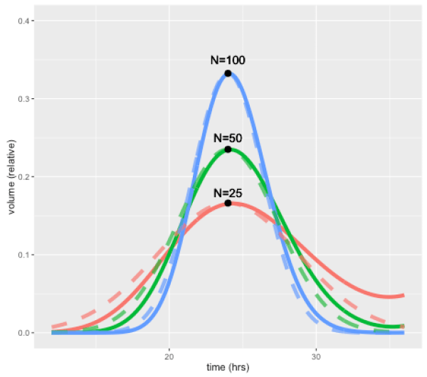
This effect is illustrated by the figure below, which shows how a perturbation at time zero in one compartment tends to blur out over time, for models with 25, 50, and 100 compartments, and a doubling time of 24 hours. In each case a perturbation is made to compartment 1 at the beginning of the cell cycle (the magnitude is scaled to the number of compartments so the total size of the perturbation is the same in terms of total volume). For the case with 50 compartments, the curve after one 24 hours is closely approximated by a normal distribution with standard deviation of 3.4 hours or about 14 percent. In general, the standard deviation can be shown to be approximately equal to the doubling time divided by the square root of N.

PertSimulationPlot
The solid lines show volume in compartment 1 following a perturbation to that compartment alone, after one cell doubling period of 24 hours. The cases shown are with N=25, 50, and 100 compartments. Dashed lines are the corresponding normal distributions.

A unique feature of the CellCycler is that it exploits this property as a way of adjusting the variability of doubling time in the cell population. The model can therefore provide a first-order approximation to the more complex heterogeneity that can be simulated using agent-based models. While we don’t usually have exact data on the spread of doubling times in the growing layer, the default level of 50 compartments gives what appears to be a reasonable degree of spread (about 14 percent). Using 25 compartments gives 20 percent, while using 100 compartments decreases this to 10 percent.

Using the CellCycler

The starting point for the Shiny web application is the Cells page, which is used to model the dynamics of a growing cell population. The key parameters are the average cell doubling time, and the fraction spent in each phase. The number of model compartments can be adjusted in the Advanced page: note that, along with doubling time spread, the choice also affects both the simulation time (more compartments is slower), and the discretisation of the cell cycle. For example with 50 compartments the proportional phase times will be rounded off to the nearest 1/50=0.02.

The next pages, PK1 and PK2, are used to parameterise the PK models and drug effects. The program has a choice of standard PK models, with adjustable parameters such as Dose/Volume.  In addition the phase of action (choices are G1, S, G2, M, or all), and rates for death, damage, and repair can be adjusted. Finally, the Tumor page (shown below) uses the model simulation to generate a plot of tumor radius, given an initial radius and growing layer. Plots can be overlaid with experimental data.

CellCyclerScreenshot2
Screenshot of the Tumor page, showing tumor volume (black line) compared to control (grey). Cell death due to apoptosis by either drug (red and blue) and damage (green) are also shown.

We hope the CellCycler can be a useful tool for research or for exploring the dynamics of tumour growth. As mentioned above it is only a “toy” model of a tumour. However, all our models of complex organic systems – be they of a tumor, the economy, or the global climate system – are toys compared to the real things. And of course there is nothing to stop users from extending the model to incorporate additional effects. Though whether this will lead to improved predictive accuracy is another question.

Try the CellCycler web app here.

References:

Stephen Checkley, Linda MacCallum, James Yates, Paul Jasper, Haobin Luo, John Tolsma, Claus Bendtsen. “Bridging the gap between in vitro and in vivo: Dose and schedule predictions for the ATR inhibitor AZD6738,” Scientific Reports.2015;5(3)13545.

Green, Kesten C. & Armstrong, J. Scott, 2015. “Simple versus complex forecasting: The evidence,” Journal of Business Research, Elsevier, vol. 68(8), pages 1678-1685.